Seaborn & Matplotlib - Q & A

Click to visit the Seaborn and Matplotlib websites.

The manuscript of journal paper usually has a page width of 16 cm. As the final article has two columns, the figure for one column will have a width of 8 cm while the figure accrossing two columns will have a width of 16 cm.

Content

Set font size and figure style
- Set font size separately if you want to change it later
- Scale font size
Set figure size
Save figure
Labels in axis
- Used scientific format in the axis
Set tick
- Change tick label size and direction
Legend
Colorbar
Colour
- Seaborn
- matplotlib
Marker
- Plot markers on top of lines
Line styles

Set font size and figure style

from matplotlib import rc
rc={'font.size' : 10, 
    'font.family' : 'Arial',
    'axes.labelsize': 10,   
    'legend.fontsize': 10, 
    'axes.titlesize': 10, 
    'xtick.labelsize': 10, 
    'ytick.labelsize': 10}
sns.set(font = 'Arial', rc=rc)
sns.set_style("ticks", {'axes.edgecolor': 'k', 
                        'axes.linewidth': 1, 
                        'axes.grid': False,
                        'xtick.major.width': 1,
                        'ytick.major.width': 1})

rcParams.update({'figure.autolayout': False})

Set font size separately if you want to change it later

ax.set_xlabel('$[G^c]_{P_w}$', fontsize = 16)
ax.set_ylabel('$\lambda_{eff} / \lambda_{solid}$', fontsize = 16)
ax.tick_params(axis="both", labelsize=16)

Scale font size

sns.set(font_scale=2)

Set figure size

fig, ax = plt.subplots(1,1,figsize=(6,4))

Here, the unit of figure size is inches. So the 16*16 cm = 6.3*6.3 inch,
16*10.7 cm = 6.3*4.2 inch (aspect ratio is 6:4),
8*8 cm = 3.15*3.15 inch,
8*5.3 cm = 3.15*2.1 inch.

In jupyter notebook, I always use 6,4 and the font size set as 15.

If you want to show the figures larger in jupyter book and still good for journal paper, using the figsize=(8,6) and font size = 14. Furthermore, if you want three figures in a row, use figsize=(6,4.5) and font size = 22 or 24.

Save figure

fig.savefig(fig_dir + 'thermal-conductivity-validation.eps', 
            format='eps', bbox_inches='tight', 
            dpi=500)
fig.savefig(fig_dir + 'thermal-conductivity-validation.png', 
            format='png', 
            bbox_inches='tight', 
            dpi=500)

Sometimes, these sentence should be in the same cell of your plot when drawing graphs in Jupyter.

Labels in axis

Used scientific format in the axis

ax.ticklabel_format (axis='x', 
                     style='sci',
                     scilimits=(0,0), 
                     useOffset=False, 
                     seMathText=True)
Labeloffset(ax, label='$[G^c]_{B_n^{edge}}$', axis="x")

Set tick

Tick interval

ax.set_xticks([1,4,5]) 
ax.set_xticklabels([1,4,5], fontsize=12)

or
ax.set_yticks(list(np.arange(0.4,0.81,0.2))) or
plt.locator_params(axis='y', nbins=4) or

import matplotlib.ticker as plticker
loc = plticker.MultipleLocator(base=0.10) # this locator puts ticks at regular intervals
ax.yaxis.set_major_locator(loc)

Change tick label size and direction

plt.xticks(fontsize=12, rotation=0)

Legend

Remove the legend title in seaborn plotting

handles, labels = ax.get_legend_handles_labels()
ax.legend(handles=handles[1:], labels=labels[1:])

Set the location of legend

To use the built-in str or floats

Location String Location Code ‘best’ 0 ‘upper right’ 1 ‘upper left’ 2 ‘lower left’ 3 ‘lower right’ 4 ‘right’ 5 ‘center left’ 6 ‘center right’ 7 ‘lower center’ 8 ‘upper center’ 9 ‘center’ 10

Example:

leg = ax.legend(fontsize      = label_font_size, 
                columnspacing = 0, 
                handletextpad = 0.01,
                loc           = 'best',
                fancybox      = True, 
                framealpha    = 0.0)

To specify the location, use bbox_to_anchor Example:

leg = ax.legend(fontsize       = label_font_size, 
                columnspacing  = 0, 
                handletextpad  = 0.1,
                bbox_to_anchor = (0.45, 0.1))

Use both loc and bbox_to_anchor Example:

fig.legend([line1], ['series1'], bbox_to_anchor=[0.5, 0.5], loc='center')
fig.legend([line1], ['series1'], bbox_to_anchor=[0.5, 0.5], loc='center left')
fig.legend([line1], ['series1'], bbox_to_anchor=[0.5, 0.5], loc='center right')

The first command will put the center of the bounding box at axes coordinates 0.5,0.5. The second will put the center left edge of the bounding box at the same coordinates (i.e. shift the legend to the right). Finally, the third option will put the center right edge of the bounding box at the coordinates (i.e. shift the legend to the left).

Change the colume of legend

ax.legned(ncol=)

Colorbar

Change the range of colorbar

plt.clim(0,13)

Change the tick intervals of colorbar

cb = plt.colorbar()
cb.set_ticks([0.75, 1.25, 1.75])

or
cb.ax.locator_params(nbins=3)

Change the tick font size in colorbar

cb = plt.colorbar()
cb.ax.tick_params(labelsize=tick_font_size)

Change the label colorbar

cb = plt.colorbar()
cb.ax.set_ylabel('$G^T_{k_w}$ (mm$^2$)',  size = label_font_size)

Colour

Seaborn

Explore Seaborn colour by clicking here

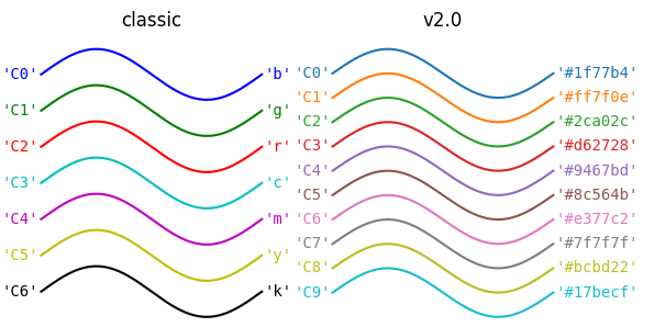
matplotlib

Explore colour by clicking here
Explore cmap by clicking here

Marker

Explore marker by clicking here

Plot markers on top of lines

using zorder

import matplotlib.pyplot as plt
x = [1,2,3,4,5,6,7,8,9]
y = [1,2,3,4,5,6,7,8,9]
plt.plot([0,10],[0,10],zorder=1)
plt.scatter(x,y,s=300,color='red',zorder=2)

Line styles

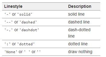
You can also set the density of the dot/dash. Click here

Latex

Remove Italic

use \mathrm
'SR$_\mathrm{ave}$'

Wenbin Fei