
Thermal Conductance Network Model
In a contact network, each node indicates a particle and an edge connects two nodes when two particles are in contact. A thermal networks is an extension of the contact network. It also considers near-contacts as edges (Fig. 1) and it can be further used to calculate the effective thermal conductivity λeff by adding thermal conductance at the edges.
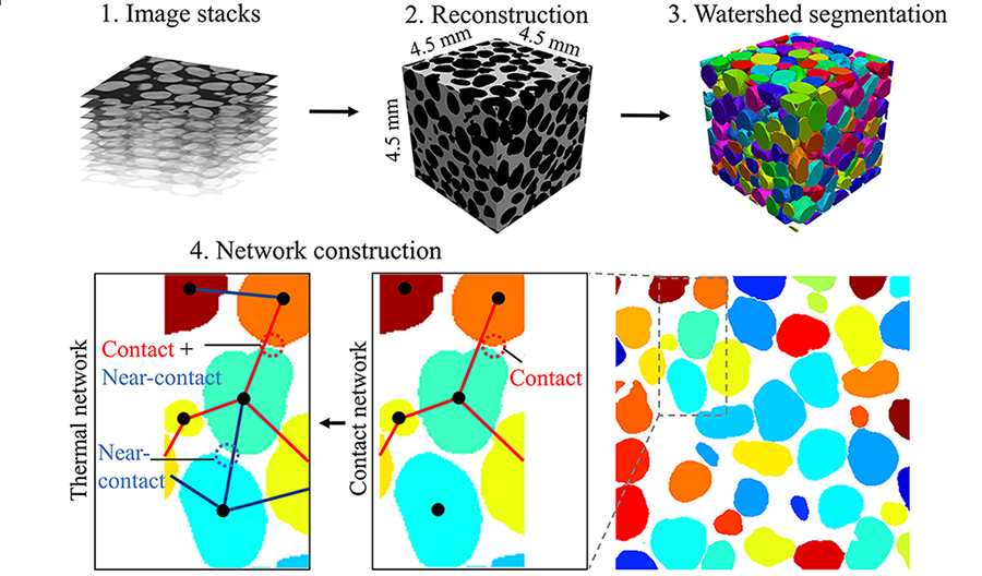
Fig.1 Procedures to construct a contact network and a thermal network. Contact edges are in red, near-contact edges are in blue.
To identify the real interparticle contact and near-contacts, the voxels in each particle are grouped as boundary voxels if they are adjacent to anything other than the voxels in the same particle. A subset of these boundary voxels is identified as interparticle contact voxels if they also border on another particle (and its corresponding boundary voxels). To efficiently identify the near-contacts, watershed segmentation is also applied to the void space (grayscale colours in Fig. 2-left) by first inverting the colour of phases and then following the same steps as with the solid phase watershed segmentation. The particle-pore connection (orange arrows) can be detected if the boundary voxels border on pore space. Then, the particle-pore-particle connections are identified as the location of potential near-contacts. Next, to determine the voxels that form part of a near-contact, cylinders representing gaps between particles or ‘gap’ cylinders are created for boundary voxels on a particle, as shown in Fig. 2-right, and their lengths Lig are computed as the minimum distance to the boundary voxels on the neighbouring particle. Finally, the gap cylinder(s) will be considered to be in a near-contact if their respective lengths are shorter than a threshold ϵ. The threshold ϵ is selected as half of the mean particle radius after a calibration.
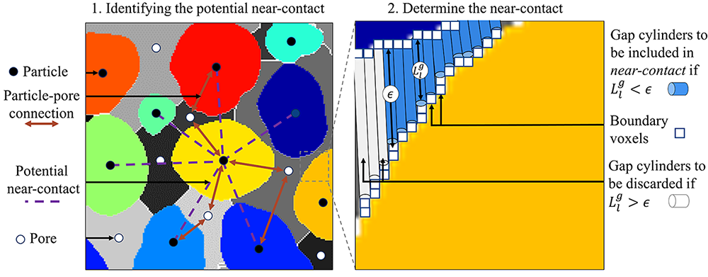
Fig.2 Identification of near-contacts. ϵ is the threshold length (D_50/4 in this case) for near-contacts.
Equivalent cylinders are used to compute thermal conductance.
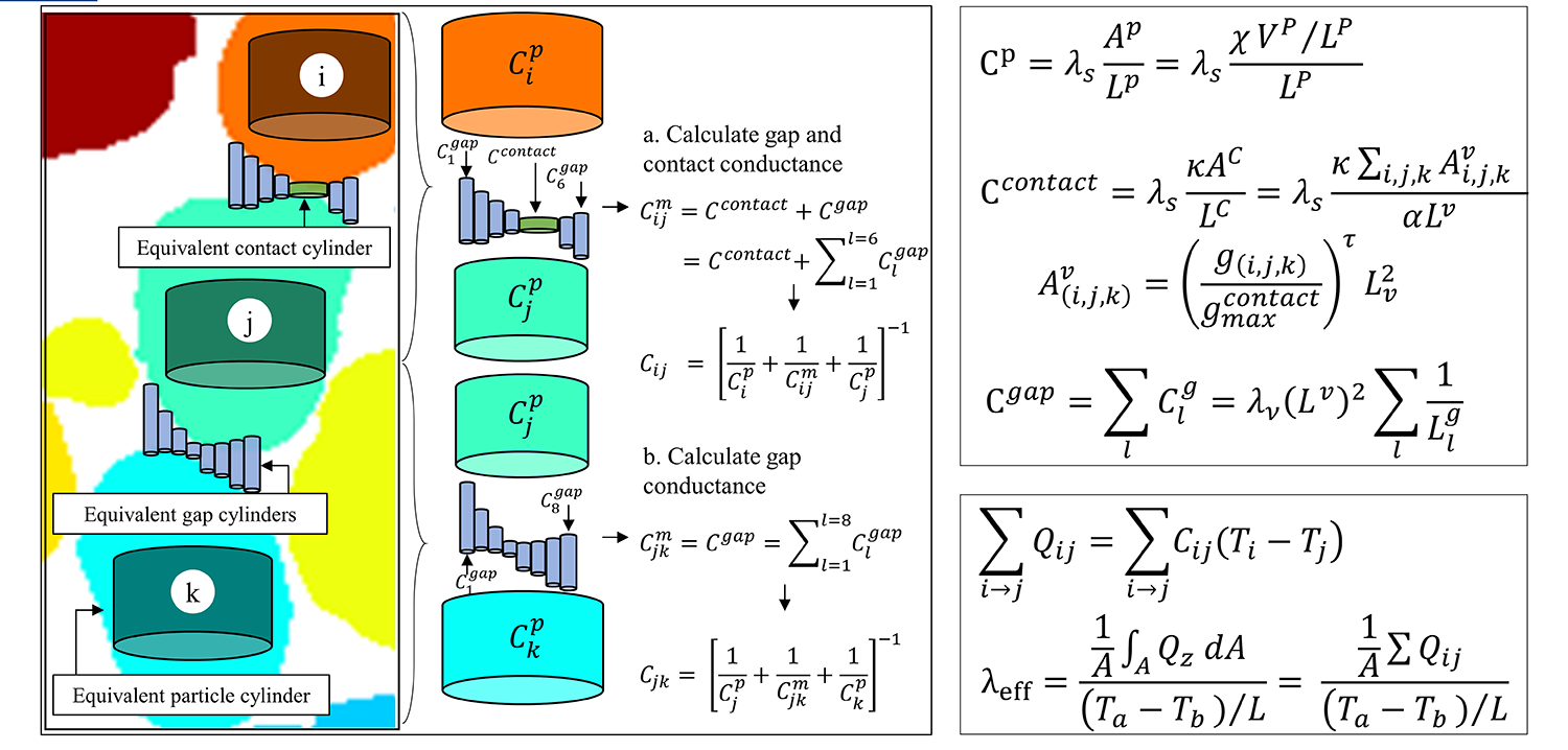
Fig.3 Computation of thermal conductance in the thermal conductance network (TCNM).
Two main advantages of TCNM are:
- Computational efficiency
- Mitigate partial volume effect
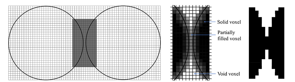
Fig.4 Over-smoothing of CT images after threshold segmentation: (a) Two discs with a 1-pixel gap; (b) a small gap in grayscale; (c) over-smoothing in the contact after threshold segmentation (after [1]).
A simulation result by TCNM is shown in Fig.5
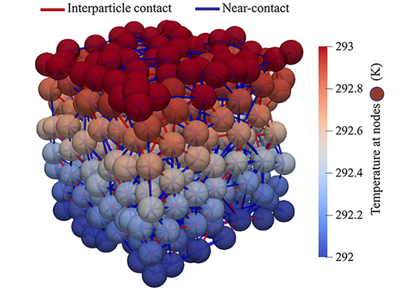
Fig.5 TCNM simulation results showing the temperature of each node. From this network system, it is easy to see paths of heat transfer: interparticle contacts are shown in red and the near-contacts are blue.
Please cite the paper below
- Fei W, Narsilio GA, van der Linden JH, Disfani MM. Quantifying the impact of rigid interparticle structures on heat transfer in granular materials using networks. International Journal of Heat and Mass Transfer 2019, 143:118514, doi
Reference
[1] M. Wiebicke, E. Andò, I. Herle, G. Viggiani, On the metrology of interparticle contacts in sand from x-ray tomography images, Measurement Science and Technology, 28(12) (2017) 124007.